Short time Fourier transform

Click to run the codes in Google colab.

Recall that a DFT takes in a time-domain signal and outputs the frequency-domain content of that signal over the entire time period of the input.

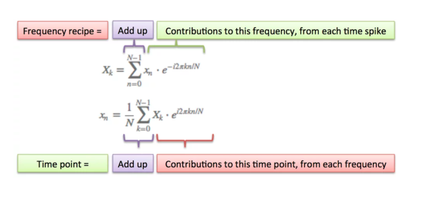
The DFT tells us about the frequency content for some signal, s. The built-in assumption, however, is that the signal's frequency content is unchanging over time.

Of course, for most "real" signals there are typically many frequency components that change over the course of the signal. Throughout the signal, then, we will need to know not only what the frequency components are, but also know when each frequency occurs. Remember: the spectrum does not contain any information about time!

The short-time fourier transform (or STFT for short) is a way of using the Fourier transform to analyze signal content that evolves over time. It works by taking very short slices of the time-based input signal and performing the DFT on each slice. With a short enough time slice, it is assumed that the frequency component(s) of that short segment is stationary, and so we can compute the DFT on that slice.

Let's look at a simple example.

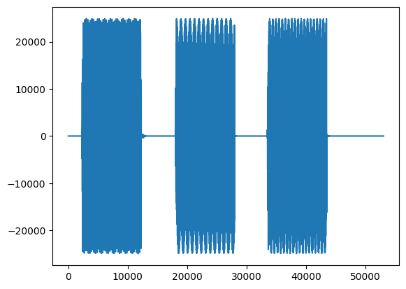
We have a signal that changes in frequency content over time, with clear stop and start positions for each tone:

                
        #import mpld3 
        #mpld3.enable_notebook() 
        from scipy.io.wavfile import read
        from scipy import signal
        import matplotlib.pyplot as plt
        #%matplotlib inline
        #%config InlineBackend.figure_format = 'svg'
        #plt.rcParams['figure.figsize'] = (9,4)
        from IPython.display import Math, Image

        fs,data = read('../audio/dialTones.wav')
        plt.plot(data)

                
        from IPython.display import Audio
        Audio(data, rate=44100)

If we run a DFT on this complete signal, we get the following:

                
        import numpy as np
        import matplotlib.pyplot as plt
        
        plt.magnitude_spectrum(data,data.size); 
        plt.xlim(0,5000) # zoomed to show relevant output

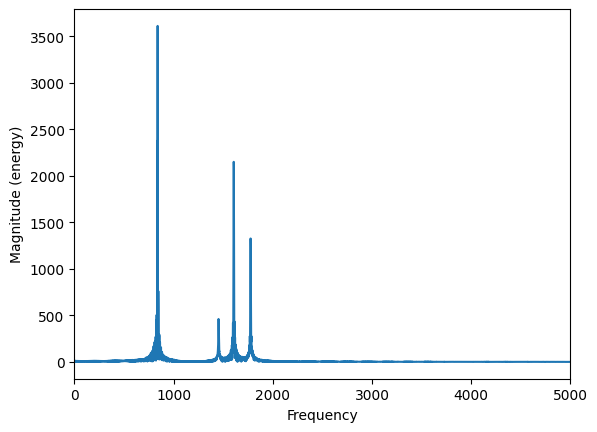
So we can see that altogether there are many different frequency components, but we don't know when they occurred. In other words, the time domain doesn't tell us about what frequencies are present, and the frequency spectrum doesn't tell us anything about when they happen.

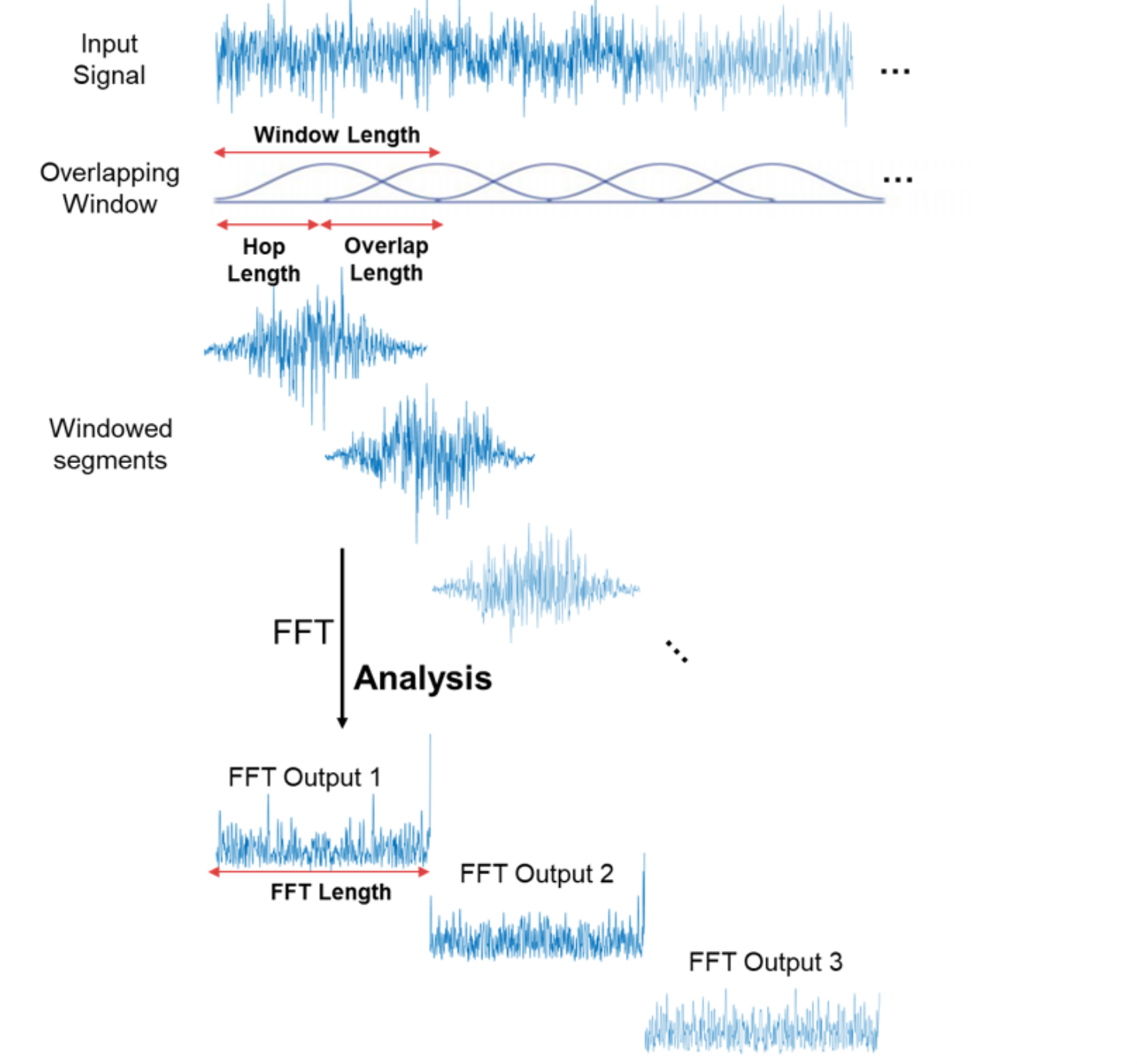
So, in order to estimate both the 'what' and the 'when', we take the audio signal, split it into small segments ("frames"), and apply a Fourier transform to each (a technique known as the short time Fourier transform or STFT). The length of this frame (snippet of time) is typically in the range of 10 to 50ms).

For reasons yet to be explained, we must apply an envelope function (i.e., "window function") to each frame of our analysis...

Thus the output $X[m,k]$ is the Fourier transform of the (typically windowed) input at each discrete time $n$ for each discrete frequency bin $k$. [More on frequency bins in a minute].

Since we are effectively computing a series of DFTs, the STFT is, (like the DFT), a complex-valued function that outputs a sequence of spetra. In other words, instead of having a vector sequnce of coefficients (what we get from the DFT), we get a matrix of coefficients, where the column index represents time, and the row index is associated with the frequency of the respective DFT coefficient.

The STFT is commonly represented as below (or some similar representation), which you should recognize as a modification of the DFT equation:

$$X[m,k] = \sum_{n=0}^{N-1} x(n + mH)w(n)\cdot e^{-j2*\pi kn/N}$$

In the above equation "m" is the frame number or frame index, and H is the "hop size" or shift lag in number of samples. $x[n]$ is now the portion of the original signal that sits inside our analysis window. $X[m,k]$ is a complex value denoting the $k$th Fourier coefficient at the $m$th time frame.

We can most easily visualize this by first applying a rectangular window across our signal:

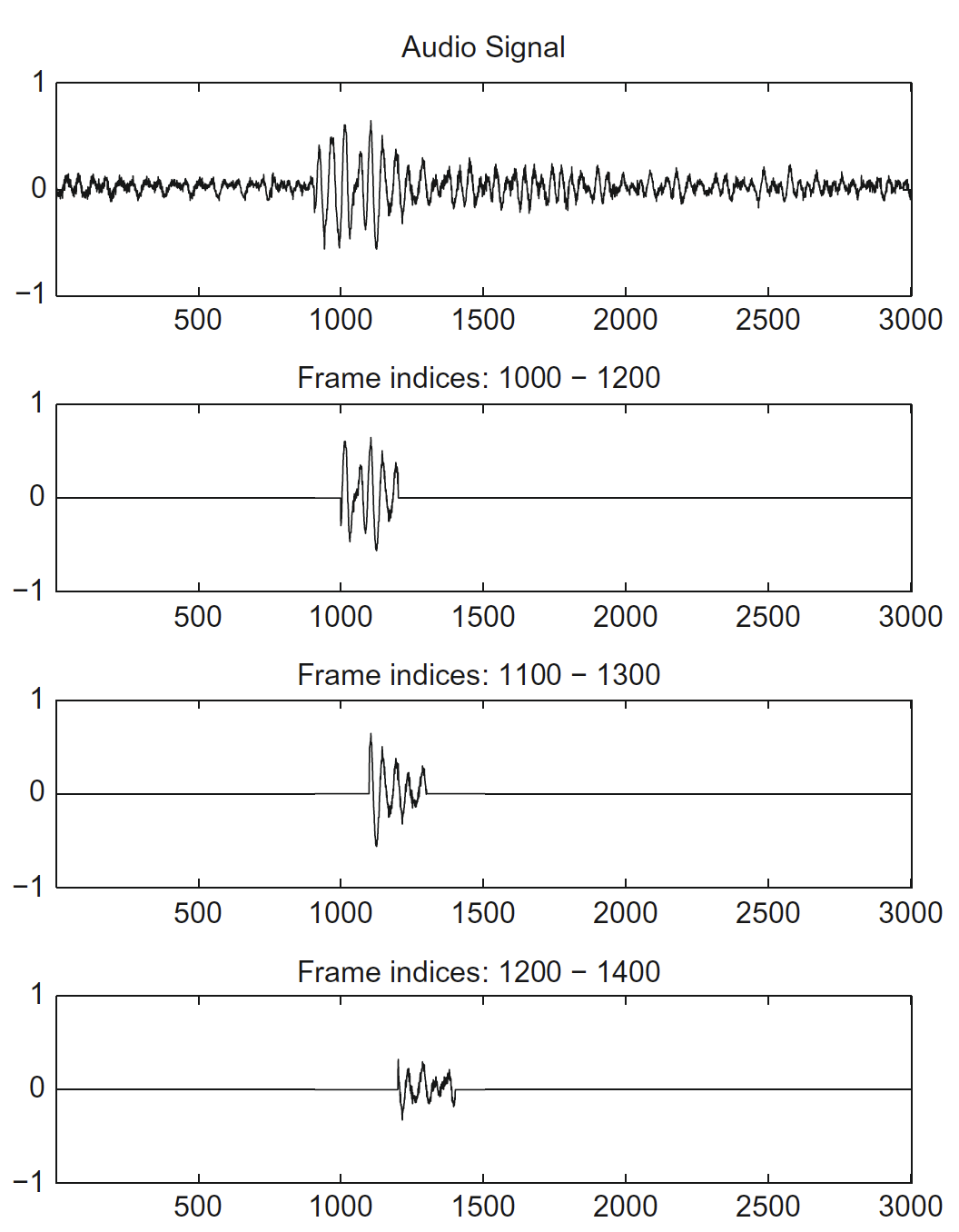
In the above example, we have a frame size of 200 (samples), and a hop size of 100 samples (i.e., 50%). A rectangular window is applied such that everything inside the window in this case is simply multiplied by 1.

So we compute a DFT over N number of samples.

Let's go back and compute the DFT for a few windows of our original example signal. (Note this is not an implementation of the full STFT because we have not windowed the entire signal but it's a good demo.)

1. N = 256 (sample 2560 to 2816) --burst one (M = 10)
2. N = 256 (sample 18,176 to 18,432) -- burst two, (M=71)
3. N = 256 (sample 37,120 to 37,376) -- burst three, (M=145)

                
        # recall our original signal here
        fs,data = read('../audio/dialTones.wav')
        plt.plot(data)

                
        f1 = data[2560:2816]
        f2 = data[18176:18432]
        f3 = data[37120:37376]
        N = f1.size
        #For now, I'm using an efficient implementation of the DFT in numpy for real-valued signals
        mx1 = np.fft.rfft(f1/N) 
        mx2 = np.fft.rfft(f2/N)
        mx3 = np.fft.rfft(f3/N)
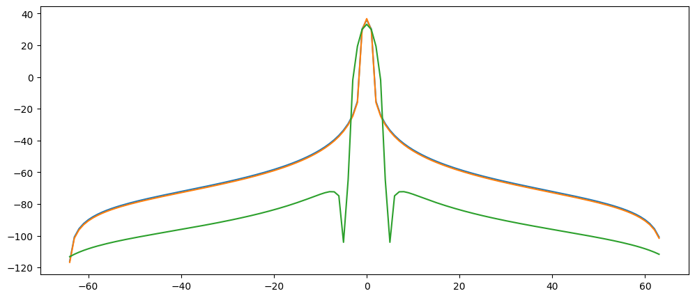
        plt.plot(abs(mx1)[:60],'r',abs(mx2)[:60],'b', abs(mx3)[:60],'g')

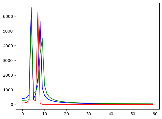
Above, each 'run' of the DFT is color-coded. The first one is red, the second blue, and the third green. You can guess that they each have the same lower harmonic component because the spikes overlap (we only see the last color -- green), but the upper component is getting incrementally higher.

Of course, here in the spectral domain those three time components are overlaid over each other because we have no way of representing time. In order to figure out *when* those time periods happened, we would need to know the number of samples passed at the beginning of our analysis frame, and the sample rate...

Recall from the DFT assignment that the number of $k$ (frequency) bins available to you was limited by the length of the input and the sampling rate. E.g., if your N was 64 then you could not find frequency components above k=64 (in fact, for a real-valued input signal, above k/2 or k=32).

So we have been looking at segments where the assumption is that the full periodicity of the signal completes during the course of the window (so say, N=64 and k=7). Thus our "sampling rate" divided by N was always equal to 1 so it was convenient to think of each "bin" as incrementing by k=1 (e.g., 1hz, 2hz, 3hz, etc.)

However, the size (or resolution) of the $k$ bins is equal to the sampling rate divided by N. Therefore if we take a smaller or larger number of samples in comparison to the size of the sampling rate (or, in this case, frame size), we change the resolution of the frequency bin such that it no longer increments by 1.

Let's keep this in mind as we continue...

Spectrogram

The spectrogram is a useful tool for capturing and visualizing this time varying spectral information. Since we are looking at very small windows of time, and most often our signal will be varying more rapidly over time (compared with our example) the above method will not be useful.

In order to represent this multidimensional data, we color code the magnitude of the fourier tranform, where large values are light or bright, and small values are dark.

We then lay these spectral "slices" one over top the other to form bands or rows of spectral data.

One way of plotting the spectrogram is with matplotlib's function:

                
        #matplotlib actually carries out the fourier transforms for you from your original signal
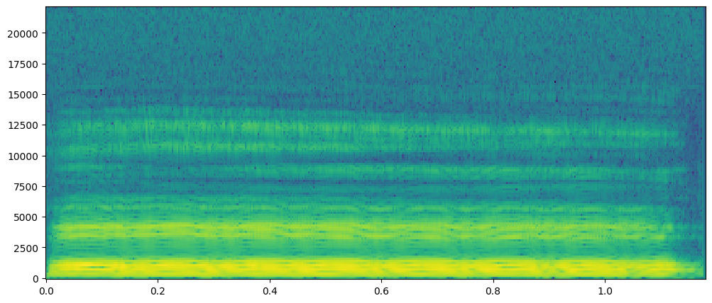
        plt.specgram(data, NFFT=256, Fs=44100) 
        plt.xlabel('Time')
        plt.ylabel('Frequency')

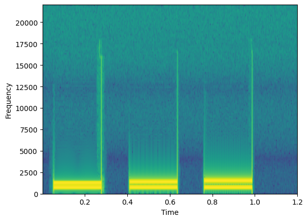
Here is an example of our frequency content over time. We can see the bright yellow bands correspond to the frequency components of each sound burst.

Notice our axis can be plotted with regard to the original time of the signal (because it's the same length).

A question that might come to mind at this point is:

What about the length of the analysis window?

Above I chose a window length of 256. Why? Is it the optimal size? What happens if we choose a larger window or a smaller window?

Recall that when we compute a DFT it is assuming a periodic signal. So we are "chopping up" the signal in an STFT hoping to find small segments that don't vary much in frequency content.

However, many times, the signal in a given window may have frequency components that have not have traversed an integer number of periods. Therefore, the finite-ness of the measured signal may result in a truncated waveform with different characteristics from the original continuous-time signal, and the artificial abrupt "cutting off" of the signal at the end of the window can introduce sharp transition changes into the measured signal.

This can create spurious high frequency content. It appears as if energy at one frequency leaks into other frequencies. This phenomenon is known as spectral leakage, which causes the fine spectral lines to spread into wider signals.

You can minimize the effects of performing a DFT over a noninteger number of cycles by using a technique called windowing (effectively, applying an envelope function to each window of time). Windowing reduces the amplitude of the discontinuities at the boundaries of each finite sequence.

This will minimize these high frequency artifacts.

Some common windowing functions include: rectangular, hann, blackman, blackman-harris, hamming... we will return to these later.

The most important thing to understand about the STFT is the necessary time-frequency resolution tradeoff which is related to the size of the analysis window.

Time-Frequency tiling

STFT determines a tiling of the time-frequency plane, where the size of each tile is specified by the time and the frequency resolution of the STFT.

So, as always, the highest positive frequency we can detect will be Fs/2 Hz, and the highest frequency resolution (how finely we can "resolve" any frequency components in the DFT) will be Fs/M Hz.

Suppose we choose a window size of length 256. What we have is a subdivision of the time axis into chunks that are 256 samples long, and subdivision of the frequency axis into bins where the size of the bin in Hz is equal to the sampling rate divided by N (or the maximum frequency divided by N/2) and the number of valid components (or frequency "bins") is equal to N/2 or 128. The size (or capacity) of the frequency axis "bins" determines our maximum frequency resolution. In the above example case, $44100 \div 256=172Hz$. So each bin is approximately 172Hz wide. There are 128 of these bins which brings us to $128 \times 172.265 = 22050$ which is our Nyquist limit.

If we change the length of the time window, suppose we take M=128, then we narrow the size of tile along the time axis, but we would therefore widen the size of the tile along the frequency axis. So now our maximum frequency resolution would be $44100 \div 128 \approx 344.5Hz$.

You can think of each tile below as returning a unique DFT value.

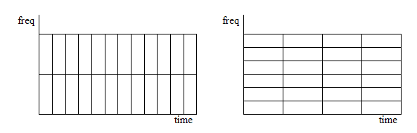
So although the shape of the tiles change, the total number of tiles remains the same, because the area of each tile remains constant.

The STFT can therefore be viewed as the output of a series of filters, or a collection of spectral sequences, each corresponding to the frequency components of $x[n]$ falling within a particular frequency band

So spectrograms can be either wideband or narrowband according to the frequency resolution of the associated DFT:

Long window: narrowband spectrogram

If our L is big, we will have more DFT points = more frequency resolution.
However, in a long window, more things can happen in the time domain = less precision in time

Short window: wideband spectrogram

short L means fewer DFT points = poor frequency resolution
short L means we capture many slices of time = precise location of transitions

If you don't have it already, pause and download the free software Audacity here

Let's have a look at the difference between a wideband and narrowband spectrogram using Audacity. If you are unsure how to get to spectrogram view in Audacity, kindly watch the short video I posted to Canvas.

Looking at files:

FemaleSingingScale.wav
chirp-150-190-linear.wav
ThreeTwoOne.wav

Listen to each of the files. The first is a simple scale with lots of space between notes, the second is a sweep with no space between tones (making it basically impossible to isolate a frequency because it is constantly changing). The last is speech only.

Look at the first two using spectrogram view. In spectrogram settings play between moving towards most narrowband (long time window) and towards most wideband (short time window). What would appear to be the best setting for each of those two files for obtaining the magnitude spectrum content?

The main disadvantage with the STFT is the uncertainty that it generates uncertainty in the frequency when the window period is too short, and, conversely, uncertainty in the time domain, when the window period is increased. This trade-off is very similar to the well-known "uncertainty principle" which is present in Quantum Mechanics.

Speech Analysis

A common use of spectrogram is in speech (and singing voice) analysis. Speech is a difficult signal to analyze. When you produce a vowel, you are producing a harmonic sound. Vowels have poor onset resolution. On the other hand, consonants have a noise-like structure, but tend to have good onset resolution. So in order to analyze a speech utterance, we need to split it into pieces and analyze them in small units.

Go back to Audacity and see if you can predict the 'noisy' consonant sounds from the harmonic vowel sounds using spectrogram in the last audio example above.

So narrowband spectrogram is useful for extracting harmonic (or vowel) sounds, hopefully you will see that while wideband spectrogram is useful for extracting information with fast-changing components such as noise-like (or consonant) sounds.

                
        import numpy as np
        import matplotlib.pyplot as plt
        plt.rcParams['figure.figsize'] = (12,5)
        from scipy import signal
        from numpy import fft
        import import_ipynb
        from IPython.display import Image, Audio

Assumptions of DFT, STFT, and Windowing

Click to run the codes in Google colab.

Recall that the DFT assumes a continuous signal. When we use a STFT, the analysis window 'cuts' the signal, and this creates an isolated DFT which assumes that the 'end' point of this cropped signal joins to the 'beginning' of it (i.e., the input is periodic and continuous). When this is false (which is usually the case), it creates sudden 'jumps' or discontinuities in the signal input. This creates artifacts in the magnitude spectrum output.

To avoid these artifacts, we typically apply a window (i.e, envelope) function to our input signal to artificially reduce these discontinuities.

"Windowing" reduces the amplitude of the discontinuities at the boundaries of each finite sequence of samples. "Windowing" consists of multiplying the time "slice" by a finite-length window with an amplitude that varies smoothly and gradually toward zero at the edges. (I.e., we are applying an envelope function that is tapered at the ends like a 'fade in' and 'fade out'). This makes the endpoints of the waveform "meet" and, therefore, results in a continuous waveform without sharp transitions.

If the amplitude of the wave is smaller at the beginning and end of the window, then the spurious frequencies will be smaller in magnitude as well.

However, since we have now multiplied to signals together (input x envelope) we will see effects of both in the spectral content. (Recall that multiplication in the time domain is equivalent to convolution in the spectral domain.

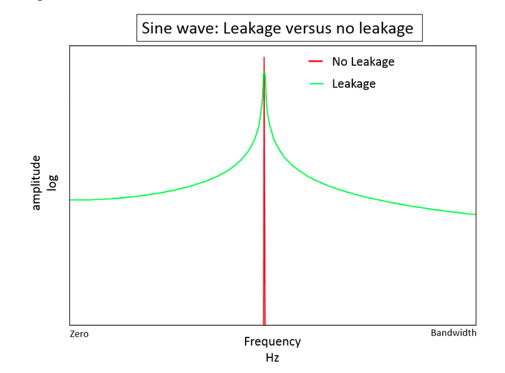
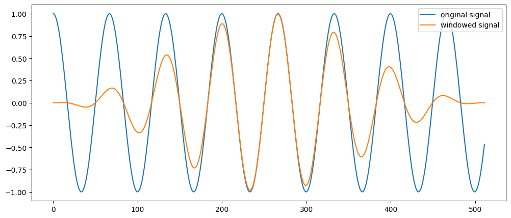
If we examine the spectrum of a single sinusoid that has been 'windowed', the spectrum you get in this case looks like a "smeared" version instead of a single peak. It appears as if energy at our one frequency component has leaked into other neighboring frequencies. This phenomenon is referred to as spectral leakage and it is typically desirable to choose a window that minimizes this leakage, while simultaneously pinpointing as accurately as possible the center frequency component.

                
        #Take a 15 hz cosine wave, grab a small fragment (512 samples) and multiply by hanning window of same size:
        w = signal.hann(512)
        t = np.linspace(0,1,1000)
        s = np.cos(2*np.pi *15 * t[0:512]) #discontinuities by cropping the signal
        line1 = plt.plot(s)
        ws = s*w # multiplication of signal with hann window
        line2 = plt.plot(ws)
        plt.legend(['original signal', 'windowed signal'])

Why are there different window "shapes"?

Windowing Functions

There are several different types of window functions that you can apply depending on the signal. To understand how a given window affects the frequency spectrum, we need to understand more about the frequency characteristics of windows.

                
        window = signal.hann(128)
        window2 = signal.hamming(128)
        window3 = signal.blackmanharris(128)
        
        plt.plot(window)
        plt.plot(window2)
        plt.plot(window3)
        
        plt.ylabel("Amplitude")
        plt.xlabel("Time Series (samples)")
        plt.legend(['hanning', 'hamming','blackmann-harris'])

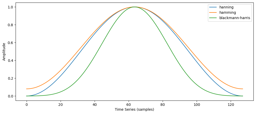
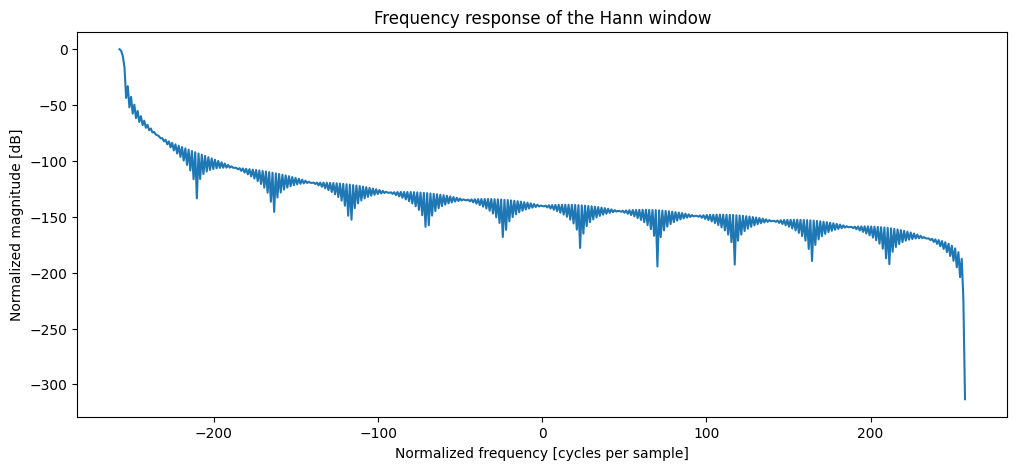
An actual plot of a window shows that the frequency characteristic of the window itself (as a signal) is a continuous spectrum with a main lobe and side lobes. The main lobe will be centered at each frequency component of the time-domain signal, and the side lobes approach zero. The height of the side lobes indicates the affect the windowing function has on frequencies around main lobes.

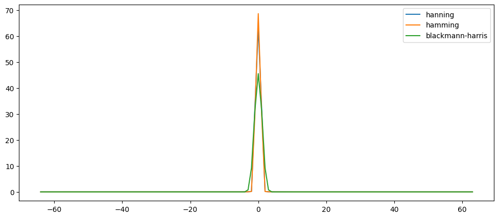
If we think of this window as an input signal, let's examine it's spectral content in isolation:

                
        from scipy.fftpack import fftshift 
        #take fft of window
        N = 128 # window size in # of samples
        Xw = np.fft.fft(window)
        Xw2 = np.fft.fft(window2)
        Xw3 = np.fft.fft(window3)
        ns = np.arange(-N/2,N/2) #center the frequencies for positive and negative components
        response = np.abs(fftshift(Xw))# plot of centered response of window -see fftshift docs-
        response2 = np.abs(fftshift(Xw2))
        response3 = np.abs(fftshift(Xw3))
        plt.plot(ns, response, ns, response2, ns, response3) 
        plt.legend(['hanning','hamming','blackmann-harris'])

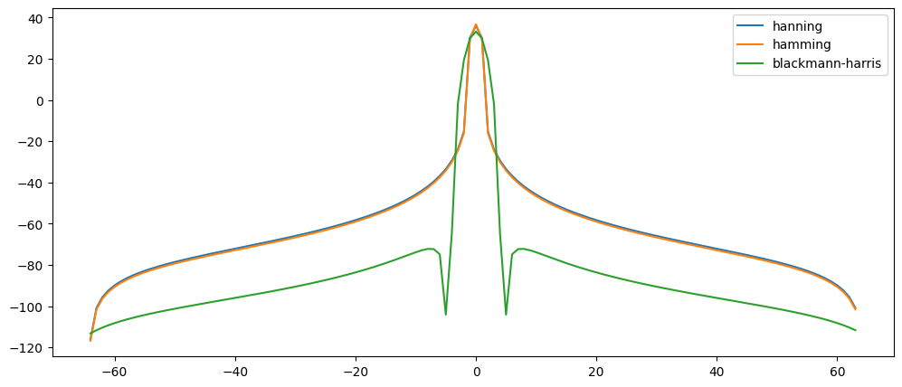
Most commonly if you read about windows and their spectral properties, it will be shown on a logarithmic scale instead of linear. Let's look at the same window on a log scale:

Choosing a window

                
        #plot on log scale to better show side lobes
        X = np.abs(response)
        X2 = np.abs(response2)
        X3 = np.abs(response3)
        
        plt.plot(ns,20*np.log10(X+0.0001/np.max(X)))
        plt.plot(ns,20*np.log10(X2+0.0001/np.max(X2)))
        plt.plot(ns,20*np.log10(X3+0.0001/np.max(X3)))
        plt.legend(['hanning','hamming','blackmann-harris'])
        #can add a tiny number to avoid error that happens when taking log of zero...

In addition, frequently you will see the log spectrum is normalized (so magnitude is divided by max magnitude):

                
        #plot on log scale; normalized magnitude - in this case it looks very similar.
        plt.plot(ns,20*np.log10(response+0.0001/np.max(response)))
        plt.plot(ns,20*np.log10(response2+0.0001/np.max(response2)))
        plt.plot(ns,20*np.log10(response3+0.0001/np.max(response3)))

STFT and Zero-padding

Sometimes we will use a segment of audio (frame) that is relatively short. We now understand that while this allows better resolution in the time domain (seeing 'when' things happen), this compromises the frequency resolution (i.e., 'where' things happen). One 'trick' to gain increased frequency resolution for shorter slice of time is to use a technique called zero padding.

With zero-padding, we simply add a bunch of empty (zero-valued) samples to the end of our slice of audio. This, of course, increases the total length of the segment, giving increased frequency resolution. However, since the numbers added are all zeros, it does not harm or change the frequency content, since anything multiplied by zero will be zero.

Fast Fourier Transform (FFT)

The usefulness of the DFT was extended greatly when a fast version was invented by Cooley and Tukey in 1965. This implementation, called the fast Fourier transform or FFT, reduces the computational complexity from:

$\mathcal{O}(N^2)$ to $\mathcal{O}(N\ log_2(N))$

The FFT is efficient because redundant or unnecessary computations are eliminated. For example, there's no need to perform a multiplication with a term that contains sin(0) or cos(0).

In addition, to take advantages of certain symmetrical properties of the DFT, the FFT algorithm has to operate on blocks of samples where the number of samples is a power of 2.

FFT in `numpy` and `scipy` packages

Both numpy and scipy have FFT functions. They are very similar. Since we'll mostly be working now with STFTs, it will be important for you to understand the parameters behind your STFT function, and that the calculation will make use of the FFT (not DFT) which is why the window sizes are always powers of two.

E.g., in the numpy.fft.rfft function it takes in n as the first argument

n: Number of points along transformation axis in the input to use. If n is smaller than the length of the input, the input is cropped. If it is larger, the input is padded with zeros. If n is not given, the length of the input along the axis specified by axis is used.

Here's a handy function to find the next closest power of two...

                
        ### use zero-padding to improve frequency resolution:
        import math
        def NextPowerOfTwo(number):
            # Returns next power of two following 'number'
            return 2**(math.ceil(np.log2(number)))

The window length could be any number, if we choose 400 or 512 the fft size will be...

                
        NextPowerOfTwo(520)

1024

                
        NextPowerOfTwo(501)

512

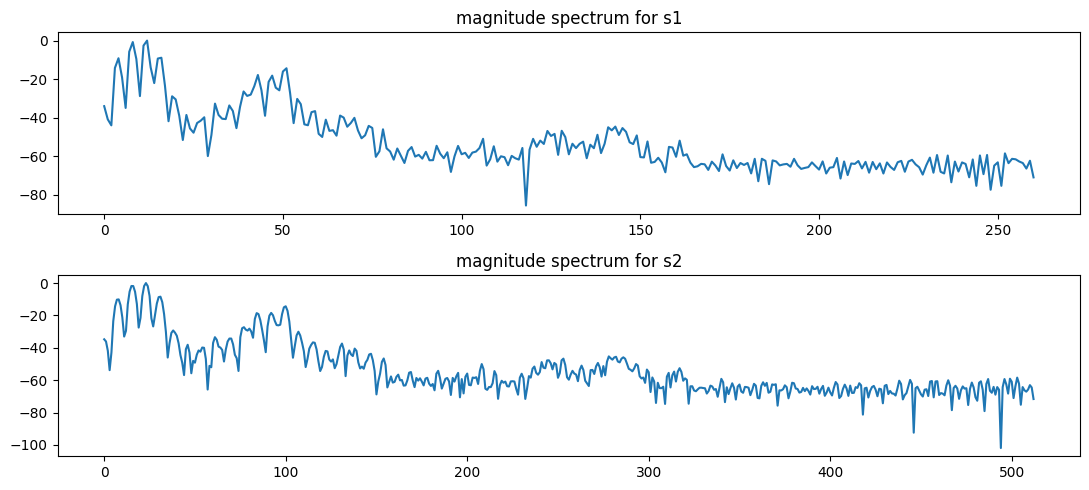
By default the rfft (fft for real-valued input) implementation will zero-pad a signal to this next power of two (or to the FFT size specified).

Zero padding results in a 'smoother' interpretation of the magnitude components.

                
        Audio('../audio/soprano-E4.wav')

                
        from scipy.io.wavfile import read
        (fs, data) = read('../audio/soprano-E4.wav')
        import numpy as np
        from numpy.fft import fftshift, rfft
        
        M1 = 520 # window size
        s1 = data[5000:5000+M1] * np.hamming(M1)  #single slice of data windowed
        pad = np.zeros(NextPowerOfTwo(M1))
        pad[:M1] = s1 # padded signal
        s2 = pad
        #s2 = np.concatenate((s1, pad)) # padded signal
        X1 = rfft(s1)
        X2 = rfft(s2)
        
        fig, axs = plt.subplots(2, figsize=(11,5))
        
        
        axs[0].plot(20*np.log10(abs(X1)/np.max(abs(X1)))) # change y-axis to db power spectrum to see more detail
        axs[0].set_title('magnitude spectrum for s1')#x-axis values are bin indices, not frequencies
        axs[1].plot(20*np.log10(abs(X2)/np.max(abs(X2))))
        axs[1].set_title('magnitude spectrum for s2')
        plt.tight_layout();

                
        window = signal.hann(526) #vary between 51 and 2048
        plt.figure()
        A = np.fft.rfft(window, 1028) # recall rfft is automatically zero-padding here...
        freq = np.linspace(-(len(A)/2),len(A)/2, len(A))
        mag = np.abs(A)
        response = 20 * np.log10(mag/np.max(mag)) #normalize amplitudes convert to dB
        plt.plot(freq, response)
        plt.title("Frequency response of the Hann window")
        plt.ylabel("Normalized magnitude [dB]")
        plt.xlabel("Normalized frequency [cycles per sample]")

Hop Size

When we apply a window to a portion of the signal, we necessarily remove content. Thus, if we align windows "end to end" there will be significant data loss. In order to minimize this data loss, we "hop" the frame (advance the window) by a fraction of its total length (usually around 50-75%). This way, when we add across the frames, we "get back" the amplitudes of the frequency components lost due to windowing.

A good rule of thum is to use 50% overlap for the rectangular window, 75% overlap for Hamming and Hanning windows, and 83% (5/6) overlap for Blackman windows.

The ideal is to have narrowest possible main lobe, and lowest side-lobe level.

Window features:

Rectangular window

main-lobe width: 2 bins (the minimum/ideal); side lobe level ~ -13db, moderate roll-off

Hamming window

main-lobe width: 4 bins; side lobe level ~ -42db, low roll-off

Hanning window

main-lobe width: 4 bins; side lobe level ~ -31db, high roll-off

Four term Blackman-Harris window

main-lobe width: 8 bins; side lobe level ~ -92db! (below noise floor - we will not hear them), moderate-high roll-off

Typically, lower side lobes reduce leakage in the measured STFT but increase the bandwidth of the major lobe. The side lobe roll-off rate is the asymptotic decay rate of the side lobe peaks. By increasing the side lobe roll-off rate, you can reduce spectral leakage. However, by increasing the width of the main lobe, you reduce the spectral accuracy by 'spreading' the energy across multiple bins.

Thus,

If the amplitude accuracy of a single frequency component is more important than the exact location of the component in a given frequency bin, choose a window with a wide main lobe.

In general, the Hanning (Hann) window is satisfactory in 95 percent of cases. It has good frequency resolution and reduced spectral leakage. If you do not know the nature of the signal but you want to apply a smoothing window, start with the Hanning window.

Plotting Spectrogram

There are several functions where you can simply pass the raw audio data and have the function compute the STFT and resulting spectrogram for you. However, it is much better if you understand what you are doing, and plot the spectrogram yourself.

Matplotlib has a plotting tool called pcolormesh which can help us do exactly this. (see here for documentation.)

                
        #read audio
        from scipy.io.wavfile import read
        (fs, data) = read('../audio/soprano-E4.wav')
        #compute STFT
        from scipy.signal import stft
        #Function args:
        '''scipy.signal.stft(x, fs=1.0, window='hann', nperseg=256, noverlap=None, 
        nfft=None, detrend=False, return_onesided=True, boundary='zeros', padded=True, 
        axis=- 1)'''
        #Note default overlap 'None' actually is 50% - see docs.
        f,t,Z = stft(data, fs=fs)
        (numbins,numspectra) = Z.shape;
        Z.shape

(129, 407)

                
        import matplotlib.pyplot as plt
        import matplotlib.colors as colors
        
        plt.pcolormesh(t,f,20*np.log10(np.abs(Z)))
        #plt.yscale('log')
        #plt.ylim(10,10**4)

ISTFT

Like the DFT, the STFT has the inverse transform. This way we can recover the original sound from the amplitude and phase spectrogram. Just like the DFT, where we overlap and add their spectra, now we we take inverse DFT of the spectral representation of every frame, and we then shift and sum ("overlap add") adding over the previous frame in such a way that we compensate for the windowing and we recover the output signal.

There are many properties to the STFT, many of which can make the ISTFT not invertible. In short, depending on the frequency resolution of the STFT, it may become non-invertible.

It is important to understand that spectrogram data is not STFT data since we are only plotting magnitude and not phase. Unlike the output of STFT, the spectrogram contains no (direct) phase information. For this reason, it is not possible to reverse the process and generate a copy of the original signal from a magnitude spectrogram alone.