Quantization
Bit Depth
Bit depth refers to the resolution of the information that gets stored in a sample. That is, it refers to the size (or length, or "depth") of numbers that can be used to store the amplitude information.
A digital audio sample is measured as a string of binary numbers. Just as we can get more precision by including more and more places after a decimal point for real numbers, binary representations can get more precise by adding more bits.
2 bits allows for 4 possibilities (0 and 1 at 2 locations); 3 bits allows for 8 possibilities; 4 bits has 16 options (below); 5 bits gives 32 options…. And it doubles each time.
| Decimal | 0 | 1 | 2 | 3 | 4 | 5 | 6 | 7 | 8 | 9 | 10 | 11 | 12 | 13 | 14 | 15 |
| Hex | 0 | 1 | 2 | 3 | 4 | 5 | 6 | 7 | 8 | 9 | A | B | C | D | E | F |
| Binary | 0000 | 0001 | 0010 | 0011 | 0100 | 0101 | 0110 | 0111 | 1000 | 1001 | 1010 | 1011 | 1100 | 1101 | 1110 | 1111 |
So the size of the binary representation we use to store audio information is referred to as bit depth, which divides the possible range of amplitudes.
4-bit = $2^4$ = 16 divisions of the amplitude
8-bit = $2^8$ = 256 divisions
16-bit = $2^{16}$ > 65.5K divisions
24-bit = $2^{24}$ > 16M divisions
16 bit audio is standard for CDs. 24 bit is standard for recording in high definition audio. At 24-bit we can cover a whopping 144dB of dynamic range!
If we look at the possibilities for how numpy can represent numbers, we can see:
| Numpy Type | C Type | Description |
| numpy.int8 | int8_t | Byte (-128 to 127) |
| numpy.int16 | int16_t | Integer (-32768 to 32767) |
| numpy.int32 | int32_t | Integer (-2147483648 to 2147483647) |
| numpy.int64 | int64_t | Integer (-9223372036854775808 to 9223372036854775807) |
| numpy.float32 | float | |
| numpy.float64 / numpy.float_ | double | Note that this matches the precision of the builtin python float. |
| numpy.complex64 | float complex | Complex number, represented by two 32-bit floats (real and imaginary components) |
| numpy.complex128 / numpy.complex_ | double complex | Note that this matches the precision of the builtin python complex. |
Because we are taking discrete measurements, the amplitude of a given sample must be rounded to the closest available value. If we had 2-bit resolution, for example, we would only have four categories for representing the amplitude (0,1,2,3; represented in binary as 00,01,10,11).
Let's look at an example:
        import numpy as np
        import matplotlib.pyplot as plt

        def f(t):
            return np.cos(2*np.pi*t)

        t1 = np.arange(0.0, 5.0, 0.1)
        t2 = np.arange(0.0, 5.0, 0.05)
        plt.figure(figsize=(10,5))
        plt.rc('font', size=20) # controls default text sizes
        plt.plot(t1, f(t1), 'bo', t2, f(t2), 'k')
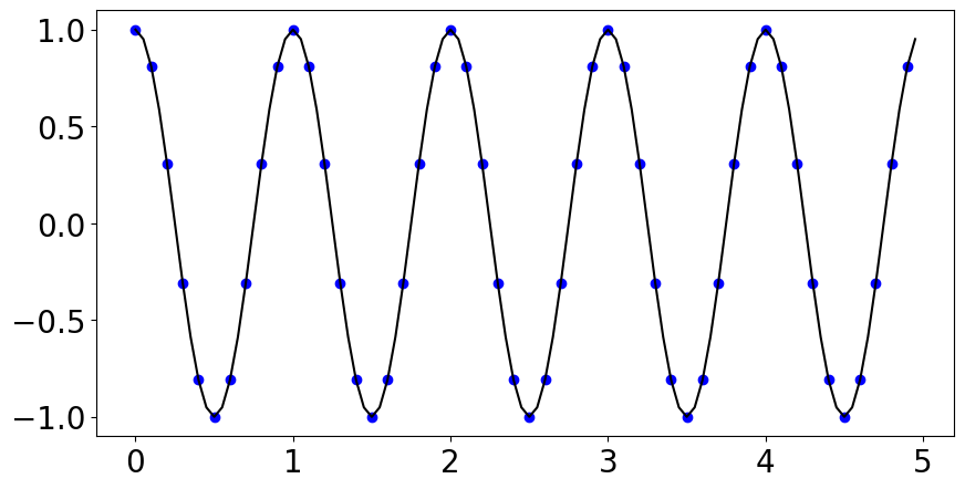
So I've sampled where the blue dots are. If we only had 2 bits (4 bins), we would have to round the actual value recorded at each blue dot to one of four equally spaced numbers between -1 and 1, and instead of the above we'd get something that looks like this:
        x = np.array([1, 1, .33,-.33,-1, -1, -1, -.33, .33, 1, 1]*5)
        plt.figure(figsize=(10,5))
        plt.plot(x, 'bo', x)
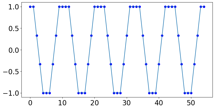
This is an extreme example because we are talking about a very low number of bits, but it makes it easy to see the distortion that could happen when the sampled values are rounded.
So the more "bins" we have for amplitude, the more accurate we can be with our numeric representations.
We get more "bins" by increasing the bit depth.
Quantization
Think of quantization as a kind of rounding or "binning" into a fixed number of discrete categories.
Just like with the last example, if we have a small number of bins to represent a large range of values, then we can think of quantization errors as "rounding errors."
A quantization error is the difference between the actual value and the rounded or "binned" value. Quantization error typically only matters when it is relatively large.
In the above example our sine wave will start to sound more like a square wave due to this quantization error arising from the reduction of the bit depth of our signal.
Quantization distortion and Dithering
Dither is a technique for dealing with something called quantization distortion. This tends to become a problem for signals recorded at very low amplitudes. These amplitudes are too small compared to the space between available quantization levels (defined by the bit depth).
In other words, you get a fairly large rounding error relative to the object's size...
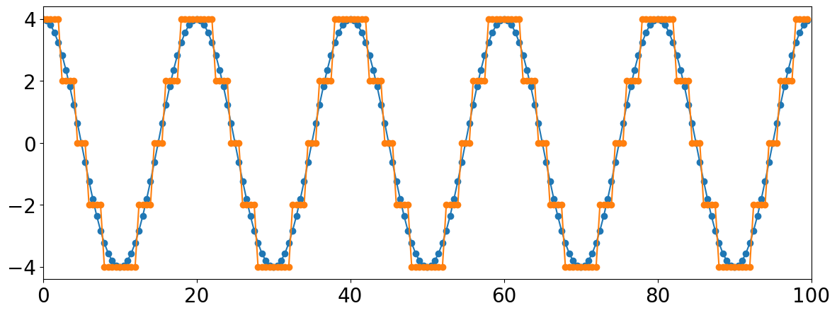
        t = np.arange(0,100,.5)
        s = 4 * np.cos(2*np.pi * 5 * t * 1/100)
        s2 = np.round(s/2) * 2

        fig = plt.figure(figsize=(14,5))
        plt.plot(t,s,t,s2,marker='o')
        plt.xlim(0,100)
        ##### t = np.arange(0,100,.5)
        s = np.cos(2*np.pi * 5 * t * 1/100)
        s2 = np.round(s, 0)

        fig = plt.figure(figsize=(15,6))
        plt.plot(t,s,t,s2,marker='o')
        plt.xlim(0,100)
        plt.ylim(-4,4)
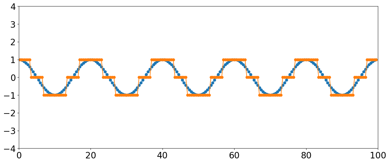
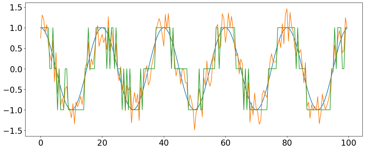
Note the large amount of quantization distortion happening for this lower amplitude signal with only 3 levels. If we reduced the signal by half, the entire thing would be rounded to zero and the signal would disappear entirely.
Dithering
Dither is typically applied when converting something from a higher resolution to a lower resolution (or bit depth), when these kinds of "rounding errors" create noticeable artifacts in the sound. Dithering is a process where one intentionally adds a very small amount of noise to the signal before quantization.
If we now quantize this messy signal with the noise added, the sinusoidal signal can still be extracted statistically from the noise. The noise smooths-out the transition between bit levels, eliminating the threshold problem.
When used in recording, the actual amount of noise added is very tiny and not noticable in the final mixed sound.
If you are using a sound recorded in 24-bit, you have so many quantization levels for amplitude that you are practically guaranteed never to have quantization distortion. However, it can become an issue when noise "adds up" from repeated signal processing, is sometimes noticable on 16 bit recordings, especially in lower amplitude ranges (~ -60dBFS).
File Type
OK, this brings us to file types and the storing of audio information. So if we thought about the uncompressed sound stored on a CD, for example, there are 16 bits of information for every sample per channel!
So assuming two channels, and a sample rate of 44,100 that's 44100 * 16 * 2 = 1,411,200 bits or ~1411 Kbits of data per second. The amount of data per second is known as the bit rate.
Computers used to be a lot slower and had less space. So in order to store it or transfer over internet, audio files needed to get smaller. So different mathematical algorithms appeared for compressing files. Depending on the method, it was translated into something called a codec.
A full quality uncompressed file like a .wav file would have a codec applied and result in a smaller file, like an MP3.
MP3s for example, at highest quality have a bit rate of approximately 320 Kbits/s.
(Codec stands for compression/decompression)
OK, so what are some ways we could reduce the amount of information in the original file?
1) Adjust sample rate. In order to scale back the size of the information per second, we would have to cut the sample rate by an order of around four.
However, cutting sample rate we run into a host of problems, especially if we cut it by that much. (We'll return to topic of downsampling...)
2) Reduce the bit depth. However, even reducing the bit depth to 8 would only get us to about 705 Kbits/s. So, what other options are there?
Recall our hearing range charts. Not many people can hear below around 50-60Hz and our hearing drops sharply above 15-16KHz, so one compression method simply eliminates any stored information that falls below 50Hz and above 15Khz, for example.
Most compression formats use fancy psychoacoustic models to determine which aspects of a sound we are unlikely to hear (for any number of reasons) and throw away that information in order to save space and/or transmission time.
There are two types of compression: Lossless and Lossy. The above two examples illustrate what's known as "lossy" compression because aspects of the original file are genuinely thrown away.
Common lossy file types include: MP3, ACC, and OGG.
Lossless, on the other hand, provides a kind of code or shortcut for storing data; for example, this type of code might say there are 500 zeros in a row, instead of physically storing all those zeros. The most common type of lossless file is FLAC (stands for Free Lossless Audio Codec).