Phase and Polarity of a Signal

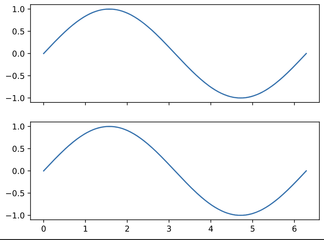
Phase is simply the position (or, more accurately, the angle) of part of a signal, and is usually calculated in radians. When two identical waveforms are superimposed, we would say that their signals are "in phase."

                
        import numpy as np
        from scipy.io.wavfile import read
        import matplotlib.pyplot as plt
        %matplotlib inline
        %config InlineBackend.figure_format = 'svg'
        
        x = np.linspace(0, 2 * np.pi, 1000)
        y1 = np.sin(x)
        y2 = np.sin(x)
        
        f, axarr = plt.subplots(2, sharex=True, sharey=True)
        axarr[0].plot(x, y1)
        axarr[1].plot(x, y2)
            #Two identical signals "in phase"
        
        #import import_ipynb
        #from #name-of-notebook import #function
                
            

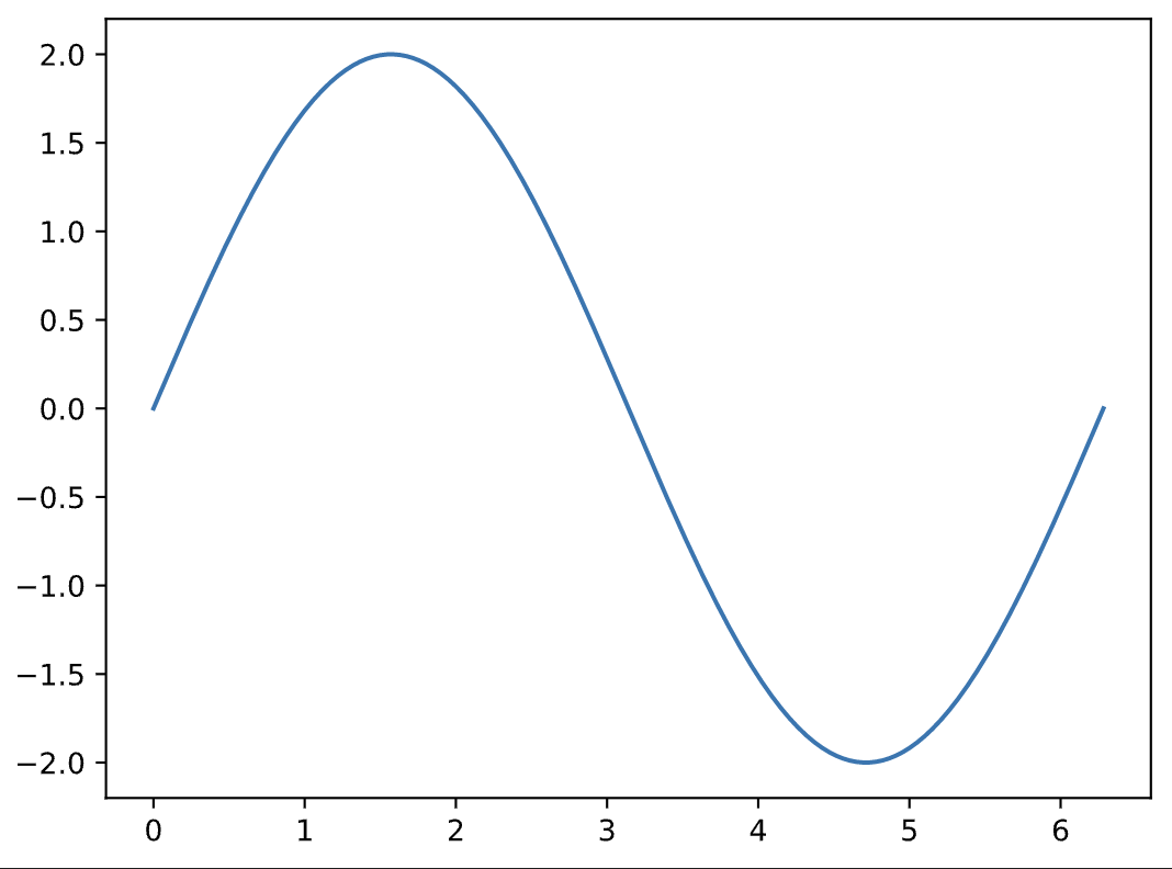
Adding these together will result in the same waveform, but just twice as loud:

                
        y3 = y1 + y2

        plt.plot(x, y3)
        #notice y-axis (amplitude) heights from above vs below
                
            

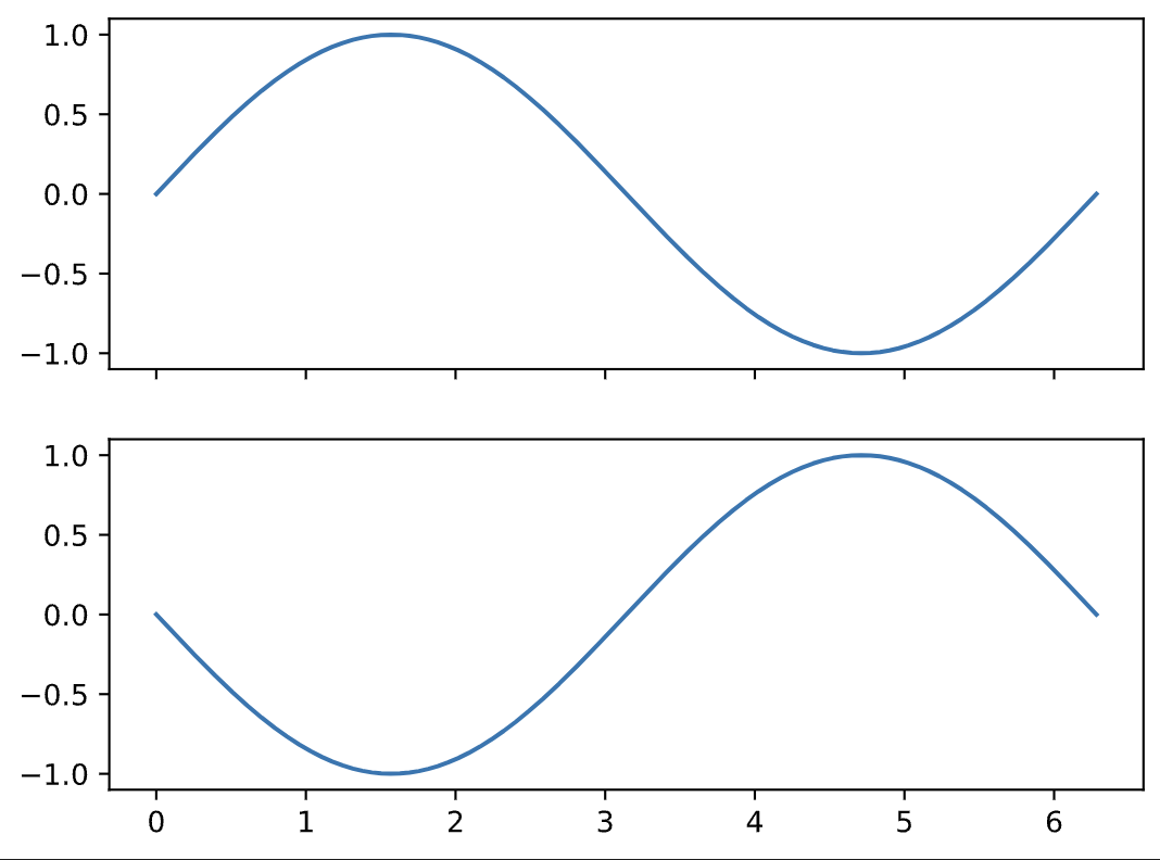
When one of the sinusoids starts at the 180º phase shift (i.e. pi radians) relative to the first this will lead to destructive interference and the result will be complete silence:

                
        x = np.linspace(0, 2 * np.pi, 1000)
        y1 = np.sin(x)
        y2 = np.sin(x + np.pi) # 2 * pi is full cycle so pi is 1/2 cycle
        
        f, axarr = plt.subplots(2, sharex=True, sharey=True)
        
        axarr[0].plot(x, y1)
        axarr[1].plot(x, y2)
            #Two signals completely "out of phase"
                
            

                
        y3 = y1 + y2

        plt.plot(x, y3)
        plt.ylim([-2, 2]) 
        # If we don't change y-lim, we get HUGE detail on y-axis and plot looks incorrect due to computer error
        #notice y-axis (amplitude) heights from above vs below
                
            

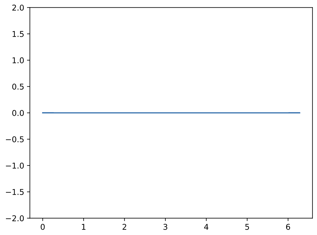
This is called destructive interference.

Now in real life this may never happen as you will not usually combine two or more waveforms that are exactly the same. Even the slightest difference between the interacting waveforms will avoid the perfect constructive or destructive interference, but some interference may still be noticeable.

If a waveform is out of phase with another waveform of similar tonality, there will be some kind of cancellation. The cancellation may not be absolute but it could be noticeable. Usually this is heard as a loss in low frequency content.

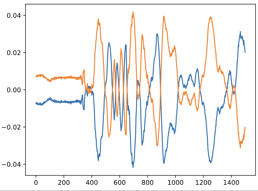
When we shift or delay the time element of a signal, we are manipulating its phase. Here, when we work with sinusoidal waveforms, the result is simple and easy to understand. If we were to manipulate a real musical signal by adding a time-varied version of itself, we would not experience the same cancellation, since the "right side" of the signal in this case will not be the inverse of the "left side" of the signal. However, we could *invert* the signal around the x-axis or amplitude domain (i.e., "flipping upside down"). If we added this version back into the original signal, we can have this same effect of destructive interference:

                
        (fs, x) = read("../audio/piano.wav")
        #normalize values to between -1 and 1:
        x = x/(np.max(np.abs(x)))
        y = -1 * x # reverse polarity of every value of x
        
        plt.plot(x[:1500])
        plt.plot(y[:1500]) #zoom in to first 1400 samples makes it clearer 
                
            

                
        z = x + y
        plt.plot(z[0:1500])
                
            

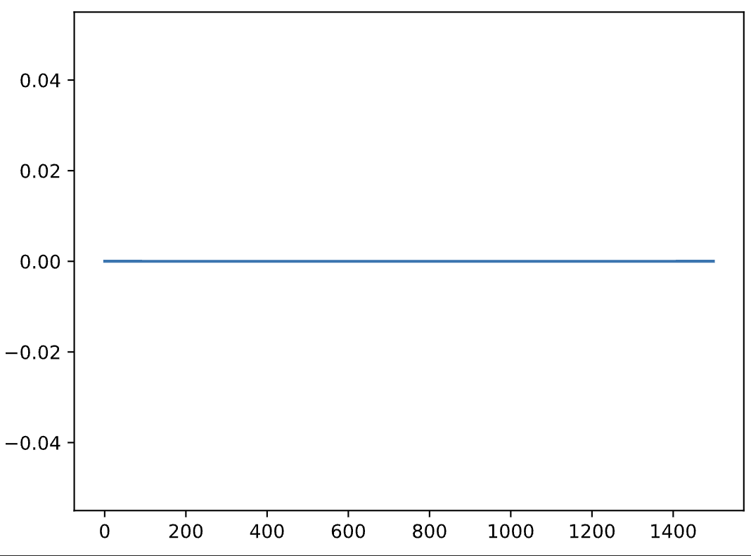
Technically, this is not phase manipulation (or "phase flipping"), but polarity manipulation (or "polarity flipping").