Modulation
Amplitude Modulation (AM)
Amplitude modulation (AM) with LFO
Just like an envelope function, we can modify one signal by multiplying it with another which will affect its amplitude over time. So a naturally smooth, time-varying signal like a sinusoid is great for creating a tremolo-like effect. One way of achieving this is with an LFO (low frequency oscillator)
This technique consists of a single multiplication of two signals: the carrier and the modulator.
The carrier wave is the original wave that we will be altering. The modulator wave refers to the wave that we will be using to alter the carrier wave. It’s more like the factor that changes the carrier wave.
More precisely, we start with a carrier oscillator and multiply by a modulating oscillator to modify and distort the carrier signal. The result is often referred to as the AM output or the "modulated" signal. However, note that (confusingly) the output is sometimes also referred to as the carrier. (So there is the original carrier and the modulated carrier).
The formula for Amplitude modulation is:
$s(t) = A_c [(1+k_a m(t))\times\cos(2\pi f_c t)]$
...where $A_c$ is the carrier amplitude, $k_a$ is referred to as the *modulator index* and $m(t)$ is the modulator signal.
The modulator is always a periodic or quasi-periodic oscillator, with a clearly defined frequency, waveshape, and amplitude.
By taking a signal oscillating at a very low frequency, and using that as our modulator frequency, we can alter a carrier signal's amplitude in a regular way. This is known as an LFO.
- The frequency of the modulator affects the rate of change of the carrier's amplitude. I.e., increasing the frequency of the modulator will increase the tremolo effect in the modulated signal.
- The amplitude (or modulator index) of the modulator affects the *depth* of change of the carrier's amplitude
- The shape of the modulator affects the regular time-varying amplitude shapes in the carrier's amplitude
We can get three different effects depending on the speed of the modulator. For a "sweep" effect we can use a very slow wave (e.g., ~0.1Hz), for a tremolo effect (e.g., 1-5Hz). If you continue to increase the speed to the upper limit of subsonic oscillations you can hear very interesting sounds including a 'growl' like sound at 10-20Hz.
        # To achieve AM all we need is a carrier and modulator that we multiply together.
        # 4 second time series
        t = np.linspace(0,4,44100*4)
        s = sawtooth(2*np.pi*80*t) #80 Hz carrier
        lfo = np.sin(2*np.pi*2*t) #2 Hz modulator
        am_out = (s*lfo) #output

        #zoom in on x-lim to better see output
        plt.subplot(3,1,1)
        plt.plot(s)
        plt.title('Carrier')
        plt.xlim(0,44100)
        plt.subplot(3,1,2)
        plt.plot(lfo)
        plt.title('Modulator')
        plt.xlim(0,44100)
        plt.subplot(3,1,3)
        plt.plot(am_out)
        plt.title('Output')
        plt.xlim(0,44100)
        plt.tight_layout()
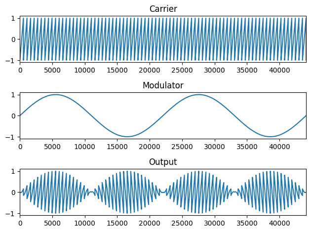
Audio(am_out, rate=44100)
Note that in order to avoid the "doubling" of the rate of modulation, we need to add a "DC offset" of 1 to the modulator wave (i.e., we need to bring all values in the modulator to positive values). This explains the "+1" DC offset in the earlier formula.
        #Example to illustrate the effect of adding DC offset:
        s = sawtooth(2*np.pi*80*t) #80 Hz carrier
        lfo = np.sin(2*np.pi*2*t) #2 Hz modulator
        am_out = (s*lfo) #output above - no DC offset
        am_out2 = ((1+lfo)*s) #DC offset included

        #5 Hz modulator, no DC offset
        Audio(am_out, rate=44100)
        #5Hz modulator with DC offset
        Audio(am_out2, rate=44100)
Notice that since the modulator ampitude touches zero this actually has the effect of "pulsing" the sound. We can change the depth of the modulator by manipulating the amplitude of the modulator (i.e., modulation index)
        am_out = (s*(1+lfo)) #adding DC offset back in to show comparison
        s = sawtooth(2*np.pi*80*t) #same 80 Hz carrier
        lfo = .5*np.sin(2*np.pi*2*t) #same 2 Hz modulator
        s_mod = (1+lfo)*s #.5 modulation index

        #zoom in on x-lim to better see output
        plt.subplot(3,1,1)
        plt.plot(s[:44101])
        plt.title('Original Carrier')
        plt.subplot(3,1,2)
        plt.plot(am_out2[:44101])
        plt.title('100% Modulation')
        plt.subplot(3,1,3)
        plt.plot(s_mod[:44101])
        plt.title('50% Modulation')
        plt.tight_layout()

        #hide_toggle()
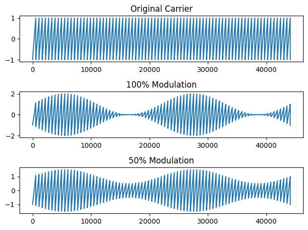
Audio(s_mod, rate=44100)
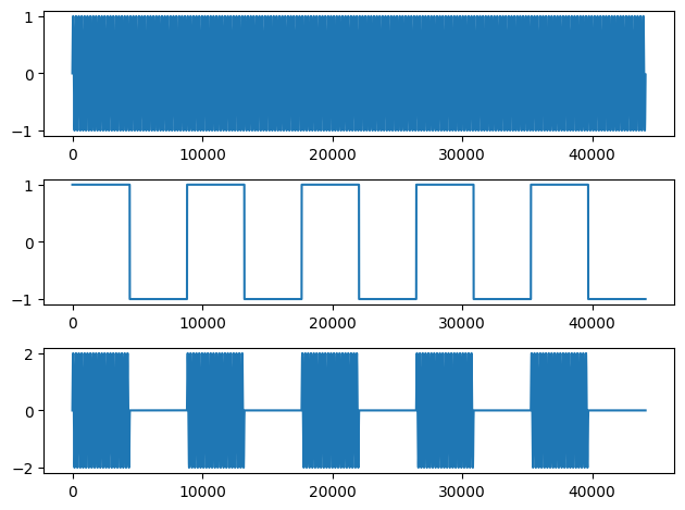
Notice that the modulating frequency does not have to be a sinusoid. Let's try with a square wave as the modulator:
        t = np.linspace(0,4,44100*4)
        s2 = sawtooth(2*np.pi*80*t) #80 Hz carrier
        lfo2 = square(2*np.pi*5*t) #5 Hz modulator - changed from sinusoid to square shape
        am_out2 = ((1+lfo2) * s2) #output

        plt.subplot(3,1,1)
        plt.plot(s2[:44100])
        plt.subplot(3,1,2)
        plt.plot(lfo2[:44100])
        plt.subplot(3,1,3)
        plt.plot(am_out2[:44100])
        plt.tight_layout()
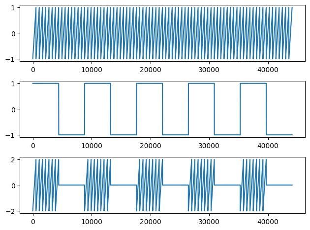
Audio(am_out2, rate=44100)
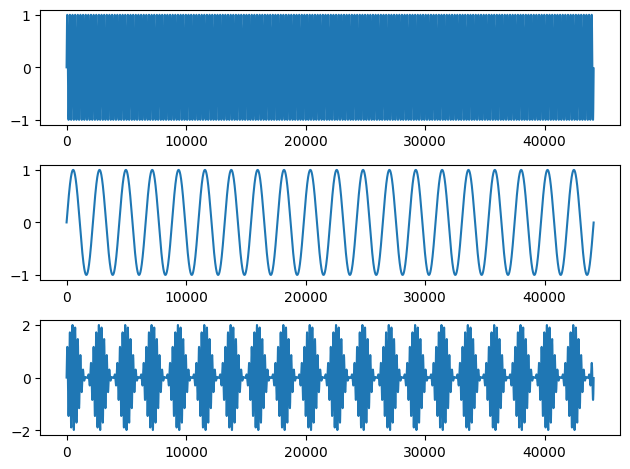
We can of course change our carrier (and modulator) to be whatever type of wave we like:
        t = np.linspace(0,4,44100*4)
        s3 = np.sin(2*np.pi*200*t) #200 Hz sinusoidal carrier
        lfo3 = square(2*np.pi*5*t) #5 Hz square modulator
        am_out3 = ((1+lfo3)*s3) #output

        plt.subplot(3,1,1)
        plt.plot(s3[:44100])
        plt.subplot(3,1,2)
        plt.plot(lfo3[:44100])
        plt.subplot(3,1,3)
        plt.plot(am_out3[:44100])
        plt.tight_layout()
Audio(am_out3, rate =44100)
Finally, notice the effect of increasing or decreasing the frequency of the modulator...
        t = np.linspace(0,4,44100*4)
        s4 = np.sin(2*np.pi*200*t) #200 Hz carrier
        lfo4 = np.sin(2*np.pi*20*t) #20 Hz modulator
        am_out4 = ((1+lfo4)*s4) #output

        plt.subplot(3,1,1)
        plt.plot(s4[:44100])
        plt.subplot(3,1,2)
        plt.plot(lfo4[:44100])
        plt.subplot(3,1,3)
        plt.plot(am_out4[:44100])
        plt.tight_layout()
        hide_toggle()
Audio(am_out4, rate=44100)
        # 200 Hz sinusoidal carrier with 10Hz triangle modulator
        # change modulator from 10 to 50

        carrier = np.sin(2*np.pi*200*t)
        modulator = 1 + 0.5 * sawtooth(2 * np.pi * 10 * t, 0.5)
        am = carrier * modulator

        plt.plot(am[:22050])
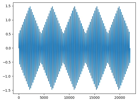
When we multiply two signals together, we combine their frequency spectra in a predictable manner. (Recall that multiplication in the time domain = convolution in the frequency domain). We have the fundamental frequency set by the carrier, but we create what are referred to as sidebands. The two sidebands are sum and difference frequencies of the carrier and modulator, C and M, and have amplitudes at half the amplitude of the carrier signal.

LFO to create tremolo for sampled sounds
We are not limited to performing AM only with basic oscillators, though. We can do it for sampled sounds too. Lets see a few examples:
Audio('../audio/bendir.wav') # Bendir is a Morroccan drum
        (fs, data) = read('../audio/bendir.wav')
        time = len(data)/fs
        t = np.arange(0,time,1/fs)
        lfo = np.sin(2*np.pi*10*t) #create 10Hz LFO same duration as input
        new_s = ((1+lfo)*data)
        Audio(new_s, rate=44100)
Audio('../audio/organ-C3.wav') # organ sound
        (fs, data) = read('../audio/organ-C3.wav')
        time = len(data)/fs
        t = np.arange(0,time,1/fs)
        lfo = .6*np.sin(2*np.pi*20*t) #12Hz LFO
        new_s = ((1+lfo)*data)
        Audio(new_s, rate=44100)
Frequency modulation (FM) and Vibrato
If AM modulation is like a tremolo effect, FM modulation when used as an LFO creates a vibrato effect.
Frequency modulation is slightly more complicated than amplitude modulation. One way of achieving the result (and allowing yourself to understand it) is with a loop function in python.
What we want to do is gradually change the frequency in Hz of the signal we are calculating as time increases. First, Here is an example of a "sweep" signal.
Let's first think about how we could change the frequency by modifying our existing formula for generating a sinusoid:
        frequency_change = 40.0
        carrier_frequency = 60.0

        fs=44100
        time = np.arange(0,3,1/fs) #time from 0 to three seconds with fs=44100

        #create carrier for graphing purposes only:
        carrier = np.sin(2.0 * np.pi * carrier_frequency * time)
        #create linear change from zero to Delta frequency:
        modulator = np.linspace(0,frequency_change,len(carrier))
        #add small increment of frequency in Hz at instantaneous time, t:
        product = np.sin(2*np.pi*(carrier_frequency+modulator)*time)

        plt.subplot(3, 1, 1)
        plt.title('Frequency Modulation')
        plt.plot(modulator) # Plot one: linear increase in frequency (i.e., the modulator)
        plt.ylabel('frequency change')
        plt.xlabel('Modulator')
        plt.subplot(3, 1, 2)
        plt.plot(carrier[:44100]) # Plot two: original frequency
        plt.ylabel('Amplitude')
        plt.xlabel('Original signal')
        plt.subplot(3, 1, 3)
        plt.plot(product[:44100]) # plot three: product of the two (i.e. Frequency modulated signal)
        plt.ylabel('Amplitude')
        plt.xlabel('Output signal')
        plt.tight_layout()
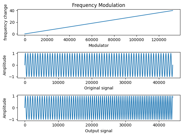
Audio(product, rate=44100)
Notice in the above function I did not actually multiply two signals together. I simply constructed a sinusoid that was modulating at an accelerating pace. To do this in a cyclical fashion (as opposed to linear), we need to alternately extend and contract the frequency or phase of the original sinusoid in order to modify each frequency cycle.
Let's define some variables:
$C$ = Carrier frequency
$M$ = Modulator frequency
$\Delta f$ = frequency deviation (or depth of modulation)
$I = \frac{\Delta(f)}{M}$ = modulation index
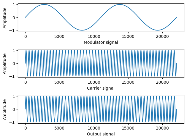
        modulator_frequency = 4 #determines periodicity of frequency shift
        carrier_frequency = 100 #determines fundamental (sometimes)
        seconds = 3.0
        I = 1.0 #determines modulation index

        time = np.arange(0,seconds*44100.0) / 44100.0  #time from 0 to three seconds with fs=44100
        carrier = np.sin(2.0 * np.pi * carrier_frequency * time) # create carrier signal for display only
        modulator = I * np.sin(2.0 * np.pi * modulator_frequency * time) # create modulator signal

        product = np.zeros(len(modulator))
        for i,t in enumerate(time):
            product[i] = np.sin(2. * np.pi * carrier_frequency * t + modulator[i])

        plt.subplot(3, 1, 1)
        #plt.title('Frequency Modulation')
        plt.plot(modulator[:22050])
        plt.ylabel('Amplitude')
        plt.xlabel('Modulator signal')
        plt.subplot(3, 1, 2)
        plt.plot(carrier[:22050])
        plt.ylabel('Amplitude')
        plt.xlabel('Carrier signal')
        plt.subplot(3, 1, 3)
        plt.plot(product[:22050])
        plt.ylabel('Amplitude')
        plt.xlabel('Output signal')
        plt.tight_layout()
Audio(product, rate=44100)
This effectively creates vibrato effect when the rate of modulation is slow (LFO).
The rate of the modulator (LFO) wave will determine the speed of the vibrato effect, and the depth (amplitude) of the modulator (relative to the carrier) will determine the intensity of the effect.
Modulator freq = rate of "vibrato" in Hz
How much the carrier deviates from its center frequency is known as the frequency deviation. The ratio of the frequency deviation to the modulating frequency is called the modulation index as defined above.
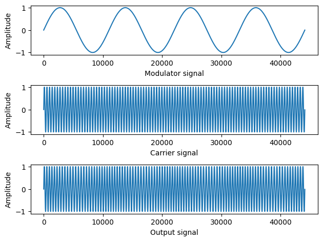
Notice that this "manual" implementation above is exactly the same as implementing FM using the familiar formula:
$Asin(2\pi C_t + Isin(2\pi M_t))$
Where the entire $Isin(2\pi M_t)$ is the phase offset term.
        modulator_frequency = 4
        carrier_frequency = 100
        seconds = 3.0
        depth = 4.0
        I = depth/modulator_frequency
        a = 1.0

        time = np.arange(0,seconds*44100.0) / 44100.0  #time from 0 to three seconds with fs=44100

        carrier = np.sin(2.0 * np.pi * carrier_frequency * time) # create carrier signal
        modulator = I * np.sin(2.0 * np.pi * modulator_frequency * time) # create modulator signal

        #rewrite above code removing loop and using FM formula:
        fm = a * np.sin(2*np.pi*carrier_frequency *time + (I*np.sin(2*np.pi*modulator_frequency*time)))

        plt.subplot(3, 1, 1)
        #plt.title('Frequency Modulation')
        plt.plot(modulator[:44100])
        plt.ylabel('Amplitude')
        plt.xlabel('Modulator signal')
        plt.subplot(3, 1, 2)
        plt.plot(carrier[:44100])
        plt.ylabel('Amplitude')
        plt.xlabel('Carrier signal')
        plt.subplot(3, 1, 3)
        plt.plot(fm[:44100])
        plt.ylabel('Amplitude')
        plt.xlabel('Output signal')
        plt.tight_layout()
Audio(fm, rate=44100)
When the modulator wave is relatively slow, we hear a vibrato effect. However, once the modulator rate increases into the audible frequency range ~20 Hz we begin to instead hear a change in the timbre of the sound (and possibly a change in the fundamental frequency). Below we will experiment with the relation between the rate of the modulator wave (M) and the carrier wave (C) in addition to the modulation index (I).
Recall:
$I = \frac{\Delta f}{f_{mod}}$ = modulation index
or
$\Delta f = I * f_{mod}$ = Depth of modulation
We could construct our FM to calculate the modulation depth based on a fixed modulation index instead of manually passing a depth value.
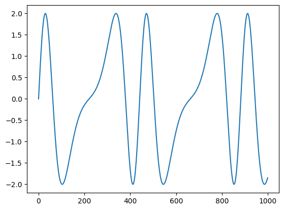
As $I$ increases, we increase the bandwidth of the spectrum (i.e., we get richer and richer sounds). These additional harmonic components will appear at intervals of $C\pm M$
        modulator_frequency = 100 #determines periodicity of frequency shift
        carrier_frequency = 200 #determines fundamental (sometimes)
        seconds = 4.0
        I = 1.78
        depth = I * modulator_frequency #determines frequency variation
        a = 2.0 #determines carrier amplitude

        time = np.arange(0,seconds*44100.0) / 44100.0  #time from 0 to three seconds with fs=44100

        carrier = np.sin(2.0 * np.pi * carrier_frequency * time) # create carrier signal
        modulator = I * np.sin(2.0 * np.pi * modulator_frequency * time) # create modulator signal

        fm = a * np.sin(2*np.pi*carrier_frequency *time + (I*np.sin(2*np.pi*modulator_frequency*time)))

        #carrier only
        Audio(carrier, rate=44100)
        plt.plot(fm[:1000]);
        Audio(fm, rate=44100)
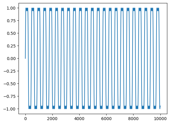
By increasing the modulating frequency so that the ratio relative to the carrier is no longer an integer multiple, an inharmonic spectrum is produced:
        modulator_frequency = 200 #determines periodicity of frequency shift
        carrier_frequency = 100
        seconds = 3.0
        I = 1
        depth = I * modulator_frequency
        a = 1.0 #determines carrier amplitude
        time = np.arange(0,seconds*44100.0) / 44100.0  #time from 0 to three seconds with fs=44100

        carrier = np.sin(2.0 * np.pi * carrier_frequency * time) # create carrier signal
        modulator = I * np.sin(2.0 * np.pi * modulator_frequency * time) # create modulator signal
        fm = a * np.sin(2*np.pi*carrier_frequency *time + (I*np.sin(2*np.pi*modulator_frequency*time)))
        plt.plot(fm[:10000]);
        Audio(fm, rate=44100)