Autocorrelation

Tempo Estimation

The beat (or pulse) of a musical piece is a periodic sequence of events or impulses. By examining the periodic structure of the impluses, we can try to estimate what one period is (the distance of a beat), which will allow us to guess the tempo.

Autocorrelation

We have learned about correlation. Autocorrelation is used to find how similar a signal, or function, is *to itself* at a certain time difference, which is referred to as lag.

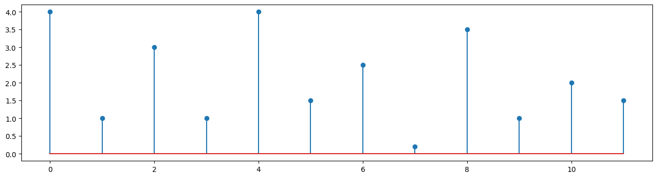
For example, let's say I have the following sequence:

                
        vals = np.array([4,1,3,1,4,1.5,2.5,0.2,3.5,1,2,1.5])
                
            

Let's make a plot to see it better:

                
        plt.stem(vals, use_line_collection=True)
                
            

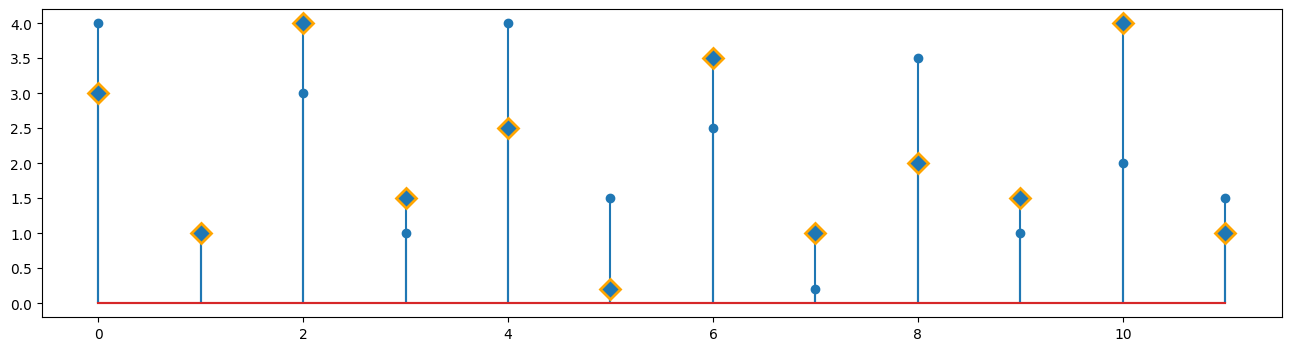
An autocorrelation will compare this original array to every possible shifted version of itself.

                
        a = np.roll(vals, -1)
        b = np.roll(vals, -2)
        c = np.roll(vals, -4)
        
        plt.stem(vals, use_line_collection=True)
        (markers, stemlines, baseline) = plt.stem(b, use_line_collection=True)
        plt.setp(markers, marker='D', markersize=10, markeredgecolor="orange", markeredgewidth=2)
                
            

                
        np.corrcoef(vals, c)
                
            

array([[1. , 0.8598234],
[0.8598234, 1. ]])

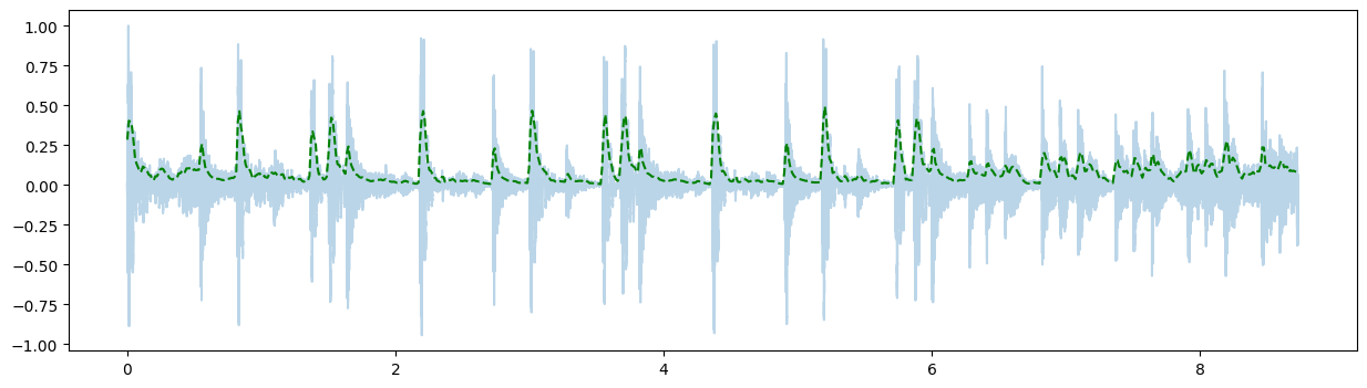
Test it out on Energy values

                
        (fs, x) = read('../audio/80sPopDrums.wav')
        xnorm = x/np.abs(x.max())

        time = np.arange(0,xnorm.size/fs,1/fs)
        hop_length = 512 # 50% overlap
        frame_length = 1024

        energy = feature.rms(xnorm, hop_length=hop_length, frame_length=frame_length)
        len(energy[0])
                
            

752

                
        frames = range(len(energy[0]))
        t = frames_to_time(frames, sr=fs, hop_length=hop_length)
        t.shape
                
            

(752,)

                
        import matplotlib.pyplot as plt
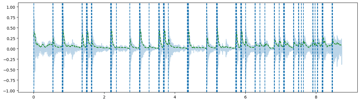
        plt.figure(figsize=(15,4))
        
        plt.plot(time, xnorm, alpha=0.3)
        plt.plot(t, energy[0], 'g--');
                
            

                
        diff = energy[0][1:] - energy[0][0:-1]
        #half-wave rectification - use numpy.where to set elements of array when condition is satisfied
        diff = np.where(diff < 0, 0, diff)
        #diff[diff < 0 ] = 0

        plt.figure(figsize=(15,4))
        plt.plot(t[1:], diff)
                
            

                
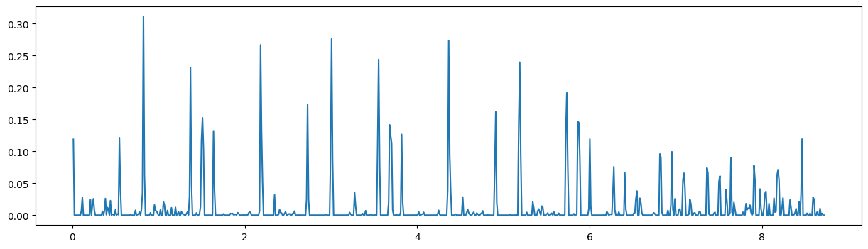
        xplines = diff > 0.03
        xplines[:20]
                
            

array([ True, False, False, False, False, False, False, False, False, False, False, False, False, False, False, False, False, False, False, False])

                
        plt.figure(figsize=(15,4))

        plt.plot(time, xnorm, alpha=0.3)
        plt.plot(t, energy[0], 'g--');
        
        for xc in t[1:][xplines]:
            plt.axvline(x=xc, linestyle='--')
                
            

                
        import librosa
        clicks = librosa.clicks(times=t[1:][xplines], sr=fs, hop_length=None)

        print(xnorm.size, clicks.size)
                
            

384993 377658

                
        clicks.resize(xnorm.shape)
        combn = clicks + xnorm

        from IPython.display import Audio
        Audio(combn, rate=fs)
                
            

                
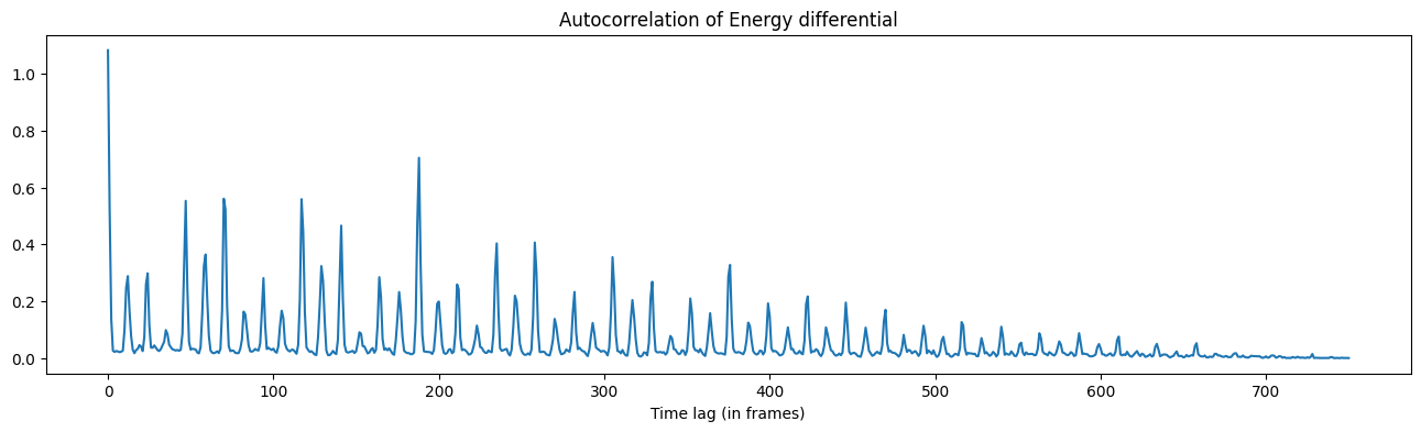
        ac = librosa.autocorrelate(diff)
        plt.plot(ac)
        plt.title('Autocorrelation of Energy differential')
        plt.xlabel('Time lag (in frames)')
                
            

                
        ac.max()
                
            

1.0824595377261215

                
        ac[0]
                
            

1.0824595377261215

                
        v = ac[1:].max()
        v
                
            

0.7043166239738892

                
        points = np.where(ac > 0.4) #ignore zero and one
        points
                
            

(array([ 0, 1, 47, 70, 71, 117, 118, 141, 187, 188, 235, 258]),)

Calculate the times between successive spikes (each frame increments by 512 samples).

                
        fsec = 512/fs
        fsec
                
            

0.011609977324263039

                
        points = np.array(points)
        t_inc = fsec * points
        # ignore first two values (zero and one)
        t_inc[0][2:]
                
            

array([0.54566893, 0.81269841, 0.82430839, 1.35836735, 1.36997732, 1.6370068 , 2.17106576, 2.18267574, 2.72834467, 2.99537415])

                
        #calculate the differences between the values
        ts = t_inc[0][2:]
        
        ts[1:] - ts[:-1]
                
            

array([0.26702948, 0.01160998, 0.53405896, 0.01160998, 0.26702948, 0.53405896, 0.01160998, 0.54566893, 0.26702948])

Notice that .011, .276, and .534 (approximately) recur (in seconds). 60 divided by these values gets us estimated tempo.

                
        tempa = 60 / .011
        tempb = 60 / .267
        tempc = 60 / .534
        
        print( tempa, tempb, tempc)
                
            

5454.545454545455 224.7191011235955 112.35955056179775

Given the "normal" range of tempi, tempc is the most likely. Check with tempo calculator.