Introduction to sounds with python
In this lesson we'll be discussing how to use python to process sounds. We will use python to read in sound files, generate sound files, manipulate sound files, and even play sound files.
Read in file as numpy array
First, we'll try reading in a sound file. To do this we'll use the scipy package, and within scipy we'll be using a module called "io" (which stands for input/output). From this module, we are going to call a function that will read in a .wav file:
from scipy.io.wavfile import read
Now we have access to the read function. For example, if we call the help function, it will give us some information about what "read" can do:
        help(read)

        #or, better, because it will open a pop-up dialog and not clog your code:
        ?read
Here we can see from the parameters that we need to pass to the `read` function (as a minimum): a string that represents the filename. Notice that it outputs two things: a sample rate, and a numpy array representing the samples of the sounds.
Note that the function will look in the same directory where your current notebook is stored for the file. If it isn't there, it will throw an error. Use the .. notation to tell Jupyter to look upwards in the directory tree for the file or ../NameOfFolder if the file is in a parallel folder.
We will call the read function on a file uploaded to the "uploaded_audio" directory (copy over from Canvas) called "Flute-A4.wav"
        (fs, x) = read("../audio/Flute-A4.wav")
        x
array([ 0, -2, 3, ..., -19, -10, -13], dtype=int16)
fs
44100
A few basics
Now we can ask some things about this file, for example, how long is the array? We do this by calling the "size" attribute:
x.size
94803
So there are 94,803 samples in the file. If we want to know how many seconds that is, we can divide by the sampling rate (44,100 samples per second):
x.size/fs
2.149727891156463
We will do more in a bit with numpy and indexing, but for now:
You can index a range of values with square brackets, like this:
x[0:100] #Gets the first 100 elements of x
        array([  0,  -2,   3,   9,  11,   6,  -2, -18, -28, -39, -37, -29, -27,

               -17, -22, -18, -18, -29, -34, -48, -58, -65, -80, -80, -75, -67,

               -57, -52, -48, -45, -39, -45, -45, -45, -44, -42, -46, -45, -46,

               -39, -37, -30, -30, -29, -36, -35, -36, -26, -17,  -9,   2,   1,

               6,   3,  17,  17,  18,  13,  11,   6,  13,  17,  24,  22,  24,

               27,  31,  33,  41,  46,  49,  53,  57,  66,  68,  70,  56,  48,

               28,  27,  24,  25,  20,  31,  31,  49,  55,  68,  68,  66,  49,

               44,  31,  26,  29,  21,  24,  23,  30,  27], dtype=int16)
Basic plotting
We can also plot the sound wave to see what it looks like. We'll do that using a popular python plotting library called matplotlib, and we'll mostly be using the pyplot module. So next, we'll import the pyplot module from the library, and give it a shortcut (or alias). Then we'll call the plot function and ask it to plot our array:
        from matplotlib import pyplot as plt
        #%matplotlib inline
        #%config InlineBackend.figure_formats = ['svg']
        import mpld3
        mpld3.enable_notebook()
        #this allows interactive plotting. "%" initiates "magic" commands.

        plt.plot(x)
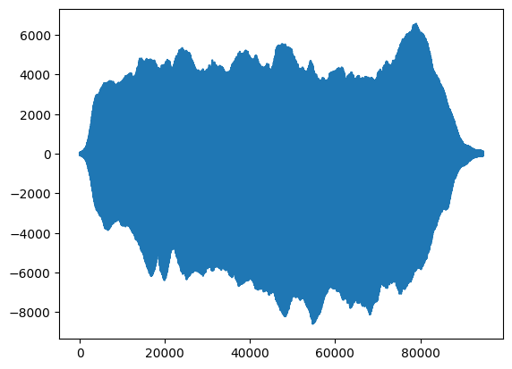
However, currently coordinates in this plot have default x-values according to their order (or "index" value; i.e., 1st, 2nd, 3rd, etc.). What would make more sense is to plot the x-axis according to time. How could we do that?
We will need to explicitly pass an array of time values to the x-axis.
We can use the `numpy` library, which is designed for working with arrays.
Specifically, we will need to convert sample positions to positions in time.
import numpy as np
We're going to use the "arange" function. Let's see what it does:
?np.arange
This is a really useful function and we'll likely be using it a lot. It creates a numpy array that begins with the "start" value, ends (before) the "stop" value, and increments by the "step" value. Notice that the "start" and "step" arguments are optional and have default values of 0 and 1, respectively.
Notice also the line about incrementing by non-integer values; in this case it's better to use the function linspace instead of arange. You can play around with them and test it out.
(You will also want to read about np.linspace, which is similar and we will also use a lot)
What will be the result of this function?:
help(np.arange)
np.arange(x.size)
array([ 0, 1, 2, ..., 94800, 94801, 94802])
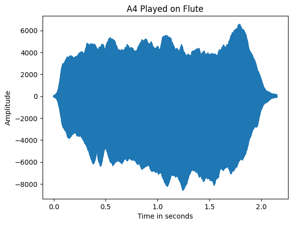
Our variable "x" is an array containing the amplitude values for every sample. Here we use np.arange to convert the array to essentially its index value (or position)--so far doing exactly what pyplot was doing by default. However, if we then divide each value by the sample rate, we will have an array representing each sample's position on a time axis beginning from zero.
        t = np.arange(x.size)/fs
        t
array([0.00000000e+00, 2.26757370e-05, 4.53514739e-05, 2.14965986e+00, 2.14968254e+00, 2.14970522e+00])
Notice that this is a vector operation (it automatically applied the division to every item in the array). Now we have a series of time values that "line up with" our sample values.
We can now redo our plot but this time plot t with respect to x:
        plt.plot(t,x)
        #matplotlib.rc('figure', figsize=(10, 5))

We should really always add titles and label our axes, so let's do that:
        plt.plot(t,x)
        plt.title('A4 Played on Flute')
        plt.xlabel('Time in seconds')
        plt.ylabel('Amplitude')
We can also play our sound back and hear what it sounds like. We'll do this by using the `Audio` function from IPython.
from IPython.display import Audio
Audio will accept many files types including mp3, but we'll only be working with wav files for now. Note that audio also accepts a numpy array. However, you should be extremely cautious before playing back any numpy arrays you have created. Always play back at very low volume first!!!
Audio('../audio/flute-A4.wav')
You can also pass Audio() a numpy array. However, you'll need to provide a sample rate as one of the arguments (or else the function doesn't know what to do)! It needs the sample rate to be able to interpret the array. Like so:
Audio(x, rate=41100)